Natural Logs with the Ln Scale

Before you do anything else, memorize this: ln(10) = 2.30.

You'll be glad. (And of course, bear in mind what I wrote in Some Terminology about the meaning of "equals" in analog computation).

With that out of the way, let's get going and see how to compute natural logarithms, that is, logarithms with base e. In this installment, we'll be using the Ln scale only (not the log-log scales found on fancier and more costly slide rules). Now Ln is not found all that commonly. Among the slide rules in my collection, only two sport it: the Pickett N1006-T, and the Pickett N4-ES. That it appears on the former is particularly attractive. This pocket unit is virtually identical to the 1006-ES I've been showing throughout here, with two important additions. First, it also includes the Ln scale. Then, all of the inverse scales are printed in red. So, this handy and pleasing rule will likely become one of my real favorites.

The place to begin with the natural logarithm is by considering its domain and range.

The domain of ln(x) is all positive real numbers. The range is all real numbers. In a manner quite similar to how we computed Common Logs, we'll find an argument on the C, D, CI or DI scale, then read the natural log from the Ln scale, adjusting the characteristic as required.

The arguments, running from 1.0 to 10.0, correspond to values of 0.0 through 2.30. We'll call these the "basic numbers," in much the same way we did for the common logarithms. These are the numbers you'll find on the opposing scales, requiring no mental adjustment for order of magnitude. With that in mind, we can work our first problem.

Exercise 1.1: Find ln(2.5).

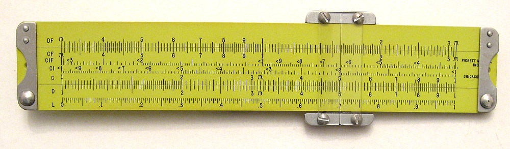
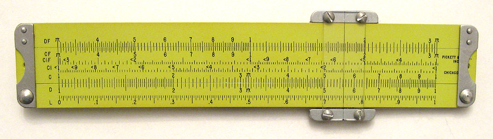
With the Pickett N1006-T slide rule I'm using, the argument is pegged on the D scale, and the associated natural log on the Ln scale. Both appear on the stator (base or stock).

We see that 2.5 is one of the basic numbers, so we can jump right in.

1. Set the cursor to 2.5 on the D scale.
2. Read the result under the hairline on the Ln scale: 0.916.

Here's how it looks on my slide rule (you can click to magnify the image):

Cursor to D:2.5, result at Ln:0.916

But what about arguments greater than 10.0, or for that matter less than 1.0? I'm glad you asked. Inspect the following figure.

In Exercise 1.1, the argument lay in the basic number span (1.0 to 10.0) which was set on the D scale. The result lay in interval 0.0 to 2.30 on the Ln scale.

Now suppose, we're searching for ln(37.2). That falls in the next interval to the right, between 10.0 and and 100.0. But consider this:

ln(37.2) = ln(10 * 3.72) = ln(10) + ln(3.72)

Of course, you already know ln(10), because I'm sure you took my advice above and memorized it, right? And 3.72 is one of the basic numbers we already know how to deal with. After a trivial sum, you'll have the desired result! Let's try it.

Exercise 1.2: Find ln(37.2).

We'll split the argument as sketched out above into a characteristic and mantissa, then press ahead.

1. Set the cursor at 3.72 on the D scale.
2. Read the number under the hairline on the Ln scale: 1.32.
3. Add this to 2.30 for the result: 3.62.

That wasn't too painful, was it?

Cursor to D:3.72, read Ln:1.32, result is 1.32+2.30=3.62

Exercise 1.3: Find ln(455).

Referring to the figure above, it should be clear that we can extend this process indefinitely to the right. Every time the argument jumps to the next order of magnitude, simply add on another 2.30. Truthfully that number is closer to 2.30256, so doubling it yields 4.61, rounded. If you'd like it spelled out for this example:

ln(455) = ln(10 * 10 * 4.55) = ln(10) + ln(10) + ln(4.55)

You'll note that 4.55 is, once more, a basic number.

1. Set the cursor to 4.55 on the D scale.
2. Read the number under the hairline on the Ln scale: 1.51.
3. Add 2.30 twice (more precisely, 4.61 once) to arrive at: 6.12.

In pictures, we have:

Cursor to D:4.55, read Ln:1.51, result is 1.51+4.61=6.12

But let's turn around and march in the opposite direction. Referring to the figure above once more, we see that for arguments below 1.0 (but greater than 0, obviously), we'll get a negative result, as expected. But think about this for a moment: arguments between 0 and 1.0 are proper fractions, and proper fractions are easily formed by the DI or CI scales.

Hence, instead of locating the argument on D, find it on DI instead, read the result off of Ln as usual, finally prefixing a minus sign. Nothing tricky at all!

One note: for a slide rule not featuring DI, simply close up the rule (aligning C with D) and use CI instead. That's what I'll be doing with the Pickett N1006-T in the pictures here, simply because CI is on the same side as Ln (DI is on the flip-side). No sense wasting energy on a duplex-flip...

Exercise 2.1: Find ln(0.25).

Here we go with a fractional argument, but larger than 0.1.

1. Set the cursor at 0.25 (2.5) on the CI scale.
2. Read the number under the hairline on the Ln scale: 1.386.
3. Prefix a minus sign: -1.386.

In summary:

Cursor to CI:2.5, read Ln:1.386, negate:-1.386

And there's no reason why we can extend this protocol further to the left.

Exercise 2.2: Find ln(0.017).

Here we have an argument one order of magnitude smaller than before. So, we'll simply subtract our magic number, 2.30, at the end.

1. Set the cursor at 0.017 (1.7) on the CI scale.
2. Read the number under the hairline on the Ln scale: 1.77.
3. Negate this: -1.77.
4. Subtract 2.30 to arrive at -4.07.

Here's how it looks:

Cursor to CI:1.7, read Ln:1.77, negate, subtract 2.30:-4.07

Now nobody is particularly fond of subtraction, but note the following. Rather than negating that 1.77 and then subtracting 2.30, why not simply add 1.77 and 2.30, then negate. Same difference, and of course it's an easy mental sum. Pretty clearly, this attack applies to any order of magnitude smaller you desire; just keep adding another 2.30 each time you drop a notch, then prefix a minus sign at the very end.

Well, I don't know about you, but I think this is all pretty cool! This little baby slide rule is able to compute any natural log, no matter the size of the argument. I still marvel that something so small, with no batteries and but two moving parts can compute products, quotients, inverses, square and cube roots, all trig functions, common logs and now natural logs...it ranks as one of mankind's most amazing inventions.

Next installment: Powers of e with the Ln Scale

Slick Approach with Folded Scales

In the previous installment, we saw that it's possible to chain a sequence of multiplications and divisions without needing to jot down intermediate results. However, from time to time, we also noticed that some rather tedious adjustments were needed to keep from going off-scale, things like index-swaps or commuting the operands. Moreover, there really were way too many slide movements in general.

We can lick all of those problems by using a slide rule which also includes the folded scales CF, DF and CIF. My little Pickett 1006-ES sports those, so that's what I'll continue using in the examples.

Of all the scales on a slide rule, the folded scales (simple as they are) perhaps provide the greatest convenience. The essential idea is that whenever an index has gone off-scale, you can do a scale-transfer to the folded scales and continue on as though nothing untoward has happened. And if that eventually takes you beyond the left or right limits, you can scale-transfer back again. Voilà! No index swapping or excessive slide movement required!

Let's try the same problems from the previous installment just to see how slick things turn out now.

Exercise 1.1: Compute 2.5 * 10.7 * 23.

If you check your notes with how we performed this chained operation last time, you'll note that it took two slide movements. Get ready to save some energy...

1. Set the cursor at 2.5 on the D scale.
2. Align 10.7 on the CI scale with the hairline.
3. Move the cursor to 23 on the CF scale.
4. Read the result under the hairline on the DF scale: 615.

Click the following photo to enlarge it and see how simple it all turns out.

Cursor to D:25, align CI:10.7 with hairline, cursor to CF:23, result at 615

Notice in step 2 we did the "divide by a reciprocal" thing to multiply by 10.7. Then immediately thereafter, searching for 23 on C revealed that it's off-scale. So instead, we find it on CF, reading the final result on DF.

As usual, at the end it was easy to estimate the order of magnitude; just think 2 times 10 times 20 = 400 and you'll know the result must be 615, not 61.5 or 6150.

This is really cool, don't you agree? Just one thing: when you do a scale transfer, do it completely. In other words, originally we were measuring with C along D. Then we migrated the pair simultaneously so CF was measuring along DF. As a general rule, never measure C against DF or CF against D (unless you have some sort of computation involving π in mind.)

For a little further practice, go ahead and find 6! (6 factorial) once more. This time you'll be able to do it with two slide movements only.

Exercise 2.1: Compute 45 / 3.8 * 75.

Here we have a mix of products and quotients, but it's just as easy.

1. Set the cursor at 45 on the D scale.
2. Align 3.8 on the C scale with the hairline.
3. Move the cursor to 75 on the CF scale.
4. Read the result under the hairline on the DF scale: 890.

Graphically we have:

Cursor to D:45, align C:3.8 with hairline, cursor to CF:75, result at DF:890

You'll note in this example, you had a choice of C or CF for that 75 in step 3. You won't always be so lucky as the next example shows. I had you use CF just for practice.

Example 2.2: Compute 45 / 3.8 * 95.

In this case, the 95 of C is off-scale to the right, so just switch over to CF and carry on.

1. Set the cursor at 45 on the D scale.
2. Align 3.8 of the C scale with the hairline.
3. Move the cursor to 95 on the CF scale. (You've no choice now!)
4. Read the result under the hairline on the DF scale: 1125.

Here's what it looks like.

Cursor at D:45, align C:3.8 with hairline, cursor to CF:95, result at DF:1125

But there's no reason to stop at three operands. We can extend this process as long as we want.

Exercise 3.1: Compute (12.5 * 37 * 0.18) / (45.2 * 11).

One of the nice things about using the folded scales is that there's no need to commute any operands for convenience sake. In this problem we'll simply multiply the three operands of the numerator in order, then divide by 45.2 and divide again by 11. Sweet!

1. Set the cursor at 12.5 on the D scale.
2. Align 37 of the CI scale with the hairline.
3. Move the cursor to 0.18 on the CF scale. (The one on C is off-scale to the left).
4. Align 45.2 of the CF scale with the hairline.
5. Move the cursor to 11 on the CIF scale.
6. Read the result under the hairline on the DF scale: 0.167.

In pictures, the steps look like this:

Cursor at D:12.5, align CI:37 with hairline, cursor to CF:0.18

Align 45.2 with hairline, cursor to CIF:11, result at DF:0.167

By this time, you should be pretty skilled at using the inverse scales. In step 2, we're dividing by a reciprocal with inverse scale CI. But in step 5 we're multiplying by a reciprocal with CIF (i.e., an actual division).

Here are a couple comments to wrap things up. First off, be sure to remember that scale-transfers are bidirectional. You can go from C/D to CF/DF or vice versa with equal ease. Anytime you're faced with an off-scale number, just switch over.

Second, Professor Herning (of whom I've referred to frequently before) has investigated the use of the folded scales for chained operations with some perspicacity. He arrived at a particularly useful rule-of-thumb: any time more than half of the slide is sticking out of the stator in chained operations, make the switch mentioned in the preceding paragraph and carry on with the alternate scales. It really works!

Be sure to spend some time with Professor Herning's excellent YouTube episode which treats chained operations with the folded scales in great detail:

Two Operations with One Slide Using Folded Scales

Were I a scientist or engineer faced with a daily deluge of computations, I'd want to be sure the slide rule I used possessed C, D, CI, CF, DF, CIF, A, B, K, S, T, ST and L at the minimum. Just so happens my favorite pocket rule, the Pickett 1006-ES has those, with a DI scale thrown in for good measure.

Next installment: Degrees, Radians and Arc Length

Basic Methods: C, D and CI

In this installment we're going to take a peep into the business of chaining various operations. We've already seen some special cases in previous episodes, most notably when dealing with squares, cubes, square roots and cube roots. But for now let's try to lay out the methods in general. Well begin with some basic techniques requiring nothing more than the C and D scales, with a pinch of CI thrown in for good measure.

Now I'm not going to kid you: by far the most elegant and most accurate approach to chaining multiplications and divisions is by means of the folded scales CF and DF used alongside C and D. However, as those aren't necessarily available on every slide rule, it makes sense to learn how to grind things out with the elementary scales as well. Even if you have the folded scales at the ready, it still pays to learn the basic methods, since they might often provide a short-circuit in the middle of a more complex computation.

As a general rule of thumb, the goal will always be to minimize the number of slide movements since each introduces a bit of dither. And we certainly want to avoid the need for writing down intermediate results or executing number-transfers from one scale to another.

Let's begin by seeing how to form the product of more than two multiplicands.

Chained Products

Here's a fact of life: with only C and D at the ready, any product of n arguments is going to require n-1 slide movements. And that's if you're lucky enough to anticipate any index-swaps in the offing. Nonetheless, this is a good way to start.

Exercise 1.1: Compute 2.5 * 10.7 * 23.

Let's jump in with both feet and simply crank this out using canonical multiplication.

1. Set the cursor at 2.5 on the D scale.
2. Align the left index with the hairline.
3. Move the cursor to 10.7 on the C scale.
4. Align the left index with the hairline.
5. Move the cursor to 23 on the C scale.
6. Read the result under the hairline on the D scale: 615.

In summary, it looks like this on my Pickett 1006-ES. You can click the pictures to enlarge them if needed.

Cursor to D:2.5. left index to hairline, cursor to C:10.7

Left index to hairline, cursor to C:23, result at D:615

You'll note that it took two movements of the slide for three operands. However, everything went according to Hoyle, and there was no need for an index-swap (nothing went off-scale). That won't always be the case as we'll see shortly.

But also observe that were was no need to write down any intermediate result, let alone even read it or know what it was. In a sense, the cursor is your scratchpad memory.

And, of course, as usual you'll need to estimate the product at the end to arrive at the proper order of magnitude for the result.

For a little extra practice, see if you can compute 6! (6 factorial, or 1*2*3*4*5*6) using this approach several times in a row. You might need the right index in places, but it's pretty easy to see it coming.

Chained Mixed Operations

The Pickett Teaching Guide for Slide Rule Instruction by Maurice L. Hartung, (Pickett, Inc.: Santa Barbara, California, 1960) recommends performing mixed operations (ones involving products and quotients) in the order: divide, multiply, divide, multiply, etc. Let's see if that's a good rule with the following.

Exercise 2.1: Compute 45 / 3.8 * 75.

1. Set the cursor at 45 on the D scale.
2. Align 3.8 of the C scale with the hairline.
3. Move the cursor to 75 on the C scale.
4. Read the result under the hairline on the D scale: 890.

Graphically, we have:

Cursor to D:45, C:3.8 to hairline, cursor to C:75, result at D:890

Hey! That only took one slide movement to carry out two operations, so Dr. Hartung's advice appears apt. Let's try the same approach on a problem which is almost the same.

Exercise 2.2: Compute 45 / 3.8 * 95.

Go ahead; give the procedure from the previous problem a try...

Uh-oh! Step 3 is problematic; that 95 is off-scale to the right. Here are some work-arounds.

Method #1: Well, it might not be our favorite thing, but let's invoke an index-swap to get past the roadblock.

1. Set the cursor to 45 on the D scale.
2. Align 3.8 of the C scale with the hairline.
3. Move the cursor to the left index on the C scale.
4. Align the right index of the C scale with the hairline.
5. Move the cursor to 95 on the C scale.
6. Read the result under the hairline on the D scale: 1125.

In pictures:

Cursor to D:45, C:3.8 to hairline, cursor to left index, right index to hairline

Cursor to C:95, result at D:1125

Compared to Exercise 2.1, that was all far from elegant, but at least it got the job done. There were two slide movements, and one of them was an index-swap. I always hate those, since with a long-range travel I just know my aging eyes or haste are going to factor in some imprecision.

You might think that can be the best you can hope for with a slide rule sporting only the C and D scales. But keep reading.

Method #2: Same problem, but let's try a different tack. What if we commute things and work towards 45 * 95 / 3.8; might that help?

1. Set the cursor to 45 on the D scale.
2. Align the right index with the hairline. (Because the next operand, 95, is so far to the right, we could anticipate and avoid the index-swap).
3. Move the cursor to 95 on the C scale.
4. Align 3.8 of the C scale with the hairline.
5. Move the cursor to the left index.
6. Read the result under the hairline on the D scale: 1125.

Here's how she goes:

Cursor to D:45, right index to hairline, cursor to C:95

C:3.8 to hairline, cursor to left index, result at D:1125

That still took two slide movements, but you'll note they weren't so extreme, i.e., the travel was considerably shorter which can only help efficiency-wise. Perhaps most important, there was no index-swap.

Method #3: For our third approach, let's see if the old "divide by a reciprocal" trick with CI has any benefits to offer.

1. Set the cursor at 45 on the D scale.
2. Align 3.8 of the C scale with the hairline.
3. Move the cursor to the left index.
4. Align 9.5 of the CI scale with the hairline.
5. Move the cursor to the left index.
6. Read the result under the hairline on the D scale: 1125. 

This is how it looks:

Cursor to D:45, C:3.8 to hairline, cursor to left index

CI:9.5 to hairline, cursor to left index, result at D:1125

Again, two slide movements were required, but just compare the photos from these three methods. In this last approach, the slide moved infinitesimally which implies you'll be burning far fewer calories if nothing else!

Okay, some of these chained operations were a little convoluted. Still, I keep coming back to: with even a simple slide rule (Rietz, Mannheim, etc.) you can do some pretty impressive things.

But if it's real elegance you crave, then lay your hands on a rule featuring the folded scales. Stop back in the next installment and you'll see how to cut all this slide movement in half.

Next installment: Chained Operations: Slick Approach with Folded Scales

Arbitrary Powers with L Only

Being able to compute a number to an arbitrary power (or take an arbitrary root) is an important skill needed by any scientific practitioner. Slide rules can do it!

Now I'm not going to kid you; raising an argument to an arbitrary number, or taking an arbitrary root of that argument is a task best left to the log-log scales...if you have them. More powerful slide rules sporting those scales make short work of such problems.

But one of the reasons I've written up this blog of techniques is to see just how much can be wrung out of a simple slide rule, like the Pickett 1006-ES I favor. With that in mind, this installment covers a method for computing powers and roots just wielding the L scale along with the usual culprits. It can be done, but requires two number-transfers, which always open up the possibility of accumulated imprecision.

I like to think of it this way. Suppose I were marooned on a desert island (which has always struck me as a curious term) and needed to find 3.5 raised to the 2.7, or the fourth root of 5. I would obviously prefer to have a Post Versalog at hand to crank things out on the log-log scales. But what if when I was stranded, only my trusty Pickett pocket slide rule survived. I could still press ahead, even if needing a couple extra steps.

So simply in the interest of squeezing as much as we can out of a basic slide rule, let's see how to conquer these more complex problems with L, a scale which appears on just about any unit.

What It's Based Upon

You'll recall from the previous two installments, we agreed to use the term basic range to mean the following. If we think of the C (or D) scale as indicating numbers between 1.0 and 10.0, then the corresponding common logarithms on the L scale span 0.0 to 1.0. (If you're a stickler for details, note that the right endpoint of either sets you back to the start again, but with a characteristic of 1 now).

For numbers outside of the basic range, either smaller or larger, we merely bring the ideas of characteristic and order of magnitude into play. Again, please refer to the previous two installments for details.

So, when tackling these new conundrums involving arbitrary exponents and roots, we'll continually reduce the numbers to lie within the basic range, simply maintaining the characteristic mentally. It's actually pretty straightforward once you've worked a couple practice problems.

The basic approach is simplicity itself, thanks to John Napier. In particular: log(b^n) = n * log(b). Crank out the right side (both the multiplication and the log are easy to do on a slide rule), then find the antilogarithm (again an easy task) and you're done.

Finding a nasty root? Then, log[b^(1/n)] = log(b)/n, take the antilogarithm and you've got it.

One last thing. Some rules put L on the slide, some on the stator. Thus you may be comparing it against C in the first case, or D in the second. A similar situation applies to CI and DI. So, in what follows, you may need to adjust the instructions accordingly depending on what style slide rule you're using.

Let's try some problems.

Argument Raised to an Arbitrary Power

Exercise 1.1: Find 3.5^2.7.

We know that the first step is to find the common log of 3.5. I'll ask you to note that this argument lies in the basic range, so we can proceed at once. However, I'll expand the instructions a bit more than in previous installments for extra detail.

1. Set the cursor at 3.5 on the D scale. This is the base.
2. Read the number under the hairline on the L scale: 0.544. This is the logarithm of the base.
3. Move the cursor to 0.544 on the D scale.
4. Align 2.7 (the exponent) of the CI scale with the hairline.
5. Move the cursor to the left index and read the product under the hairline on D: 1.47. This is the product log(3.5) * 2.7.
6. The 1 in 1.47 is the characteristic (remember it), while 0.47 is the logarithm lying in the basic range.
7. So, move the cursor to 0.47 on the L scale.
8. Read the antilogarithm under the hairline on the D scale: 2.94.
9. Finally, factor in that characteristic (order of magnitude) that you remembered to arrive at the final result: 29.4

That all sounds a lot worse than it really is as the following pictures indicate:

Cursor to D:3.5, read log L:0.544

Cursor to D:0.544, CI:2.7 to hairline, read left index D:1.47

Cursor to L:0.47, read D:2.94, interpret as 29.4

I hope it's obvious that in step 4 we were using the old "divide by a reciprocal" trick with CI to carry out the multiplication.

Run through the steps for practice a couple times, noting how that 1 in step 6 got stripped away to that we could continue on with numbers in the basic range.

In the next problem you'll need to consider the basic range at the start as well. It really isn't all that big of a deal after just a modicum of practice.

Exercise 1.2: Find 15^5.2.

1. Set the cursor at 1.5 (which with a characteristic of 1 represents 15) on the D scale.
2. Read the logarithm of 1.5 under the hairline on the L scale: 0.176.
3. Append the characteristic from step 1, yielding the complete logarithm of 1.176.
4. Set the cursor to 1.176 on the D scale.
5. Align 5.2 of the CI scale with the hairline.
6. Move the cursor to the right index.
7. Read the product under the hairline on the D scale: 6.12.
8. Thus, the characteristic of this log is 6; remember it.
9. Move the cursor to 0.12 on the L scale.
10. Read the antilogarithm under the hairline on the D scale: 1.31.
11. Factor in that characteristic of 6 (i.e., scale by 10^6): 1,310,000.

In pictures, you'll see:

Cursor to D:1.5, read log L:0.176, form complete log 1.176

Cursor to D:1.176, align CI:5.2 with hairline, read right index D:6.12

Cursor to L:0.12, read D:1.31, interpret as 1310000

I hope I haven't freaked you out with this detailed description of the steps. True, you'll be doing a couple number-transfers, but I can promise you after you've run through it all a few times, it really does become second nature if you'll only remember Napier's power rule.

Arbitrary Roots

We need to try a root problem. Everything runs pretty much the same way, except we'll be dividing that common log early on, not multiplying into it.

Exercise 1.3: Find the fourth root of 5.

1. Set the cursor at 5 on the D scale.
2. Read the logarithm under the hairline on the L scale: 0.7.
3. Move the cursor to 0.7 on the D scale.
4. Align 4 on the C scale with the hairline.
5. Move the cursor to the left index.
6. Read the quotient under the hairline on the D scale: 0.175.
7. Move the cursor to 0.175 on the L scale.
8. Read the result under the hairline on the D scale: 1.5.

You'll note in this problem that everything stayed within the basic range. Pictorially, we have:

Cursor to D:5, read logarithm L:0.7

Cursor to D:0.7, align C:4 with hairline, read left index D:0.175

Cursor to L:0.175, result (antilogarithm) at D:1.5

(While writing this up, it occurred to me that for this particular problem it would be faster and probably more accurate to simply take the square root of 5 twice with the A scale. So, keep your eyes open!)

I'll confess, there's a fair amount of slip-sliding going on with these problems. But don't you think it's cool that one can even attempt arbitrary roots and powers with just the simplest of slide rules? Give me C, D, CI, DI and L and I'm ready to conquer the world...

Next installment: Natural Logs with the L Scale

Powers of Ten

In the previous installment we saw how to compute a common logarithm: simply dial in the argument on the C, D, CI or DI scale, and read the log on the L scale. Obviously, one can turn this around to compute a power of 10. Now finding a power of 10 probably sounds exceedingly dull; I mean how often do you run into such a problem in scientific calculations?

But viewing this instead as an antilogarithm all of a sudden makes its utility clear. In the manner of Henry Briggs (the first advocate of common logs), we'll find there are a number of interesting applications in which we first convert expressions to logarithms, do some simple arithmetic, then convert that sub-tally back to a desired result via the antilogarithm.

Last time we agreed to call the span of numbers on the C or D scale the basic range, i.e., 1.0 through 10.0, with the corresponding mantissas on the L scale covering 0.0 through 1.0.

Now with powers of 10, we'll reverse gears but still call it the basic range. In short, on a slide rule the arguments for powers of 10 will lie between 0.0 and 1.0, with a result in the range 1.0 to 10.0. Dealing with arguments outside of that span is easy, just by remembering a simple property of exponents. Let's get started.

Arguments Between 0 and 1

In all of the problems to follow, you'll be starting with the L scale, then working backwards to the D scale. Depending on the arrangement of your slide rule (is L on the slide or stator?) you might be using C instead. And where reciprocals come into play, you might need CI instead of DI.

Exercise 1.1: Find 10^0.3.

1. Set the cursor at 0.3 on the L scale.
2. Read the result under the hairline on D: 1.995.

Here's how it appears on my Pickett 1006-ES pocket slide rule. As usual, you can zoom in by clicking the photo:

Cursor to L:0.3, result at D:1.995

Exercise 1.2: Find 10^(0.57).

1. Set the cursor at 0.57 on the L scale.
2. Read the result under the hairline on D: 3.72.

Graphically, we have:

Cursor to L:0.57, result at D:3.72

If you stop to think about it, we now know how to find any simple root of 10, i.e., square root, cube root, fourth root, etc.

Arguments Greater Than 1

This is really easy, recalling how addition of exponents works. For example, given 10^4.7, split this up into (10^4) * (10^0.7). You'll notice that the second factor now has an argument falling in the basic range which can be worked directly using the method just seen. Just keep the 10^4 as your order of magnitude.

And of course, once you know the reason, there's no need to actually think of the exponent rule used: simply split the number 4.7 into a 4 and a 0.7 and carry on.

Exercise 2.1: Find 10^4.7.

1. Set the cursor at 0.7 on the L scale.
2. Read the number under the hairline on the D scale: 5.
3. Form the result: 5 * 10^4.

This is how it looks:

Cursor to L:0.7, read number D:5, form result 5*10^4

Exercise 2.2: Find 10^21.5.

1. Set the cursor at 0.5 on the L scale.
2. Read the number under the hairline on the D scale: 3.16.
3. Form the result: 3.16 * 10^21

In pictures:

Cursor to L:0.5, read number D:3.16, form result 3.16*10^21

You'll note in these problems, the result is automatically shaped into scientific notation form. Nice!

Arguments Between -1 and 0

Recalling that negative arguments imply a reciprocal is on the menu, you won't be startled to learn problems like this use the DI (or CI) scale instead of D (or C).

Exercise 3.1: Find 10^(-0.75).

1. Set the cursor at 0.75 on the L scale.
2. Read the result under the hairline on CI: 0.178.

In the photo here, I'm using CI since it lies on the same side as L, thus avoiding a duplex-flip:

Cursor to L:0.75, result at CI:0.178

Now, you might be nonplussed that we ended up with 0.178 and not 1.78. After all, isn't the latter in that basic range alluded to earlier? It would be but for the fact the exponent was negative, implying a reciprocal was a-coming. So, if the basic range is 1.0 to 10.0, then the multiplicative inverses of that range (found on CI) span 1.0 down to 0.1.

Exercise 3.2: Find 10^(-0.2).

1. Set the cursor at 0.2 on L.
2. Read the result under the hairline on CI: 0.631

It looks like this:

Cursor to L:0.2, result at CI:0.631

Once again, we arrive at a number between 0.1 and 1.0.

Arguments Less Than -1

A moments reflection ought to convince you that one can combine the techniques from above to arrive at powers of 10 when the argument is less than -1. For example: 10^(-12.5) = 10^(-12) * 10^(-.5). Just press ahead with what you've already learned and you'll arrive at 3.16 * 10^(-13).

Pop Quiz: Do you understand why that exponent is -13? Think about the standard form for scientific notation.

Tiny Arguments

If the argument shrinks toward zero, then clearly the power of 10 approaches 1. In fact, it'll get so close on a slide rule that you probably ought to give up once the argument drops below 0.01. Nonetheless, just for the heck of it, let's try one that's small but not so small that we can't read it under the hairline.

Exercise 4.1: Find 10^0.038.

Now this is tricky, but do-able. We need to get things into the basic range first. So write the expression as 10^0.038 = 10^(1-0.962).

Okay, finding the complement of 0.038 as 0.962 isn't exactly automatic, but it's still a reasonable mental computation. Anyway, we can now carry on with the methods from above.

1. Set the cursor at 0.962 on L.
2. Read the number under the hairline on CI: 0.109.
3. Adjust result to 1.09 since the characteristic was 1.

Pictorially:

Cursor to L:0.962, result at CI:1.09

To repeat, we were working with an exponent of 1- 0.962 at the outset; that 1 represents the characteristic, one complete power of 10. So, at the end, we needed to factor it back in.

The domain of 10^x is all real numbers, and in the paragraphs above we have accounted for all possibilities, realizing that it always comes back to what's happening in the basic range.

Next installment: Arbitrary Powers with L Only

Common Logs with L Scale

In this set of installments, I propose we look into how to handle exponentials and logarithms, along with some of their applications. We'll begin with the L and Ln scales and wring everything out of them we can, before getting on to the log-log scales for even more dramatic doings.

The L scale is laid out to give common logarithms, i.e., base 10. Apart from their great utility in computational work, base 10 logs also pop in a broad range of applications: the pH scale in chemistry, the magnitude scale in astronomy, the Richter scale in earth science, the decibel scale in audiology, and more. Even crazier is that for centuries, astrologers used common logs when casting a horoscope!

Notably, when I took a freshman trigonometry class in college (but not as a freshman!), we used tables of common logs for all of our computations. Pocket calculators were still on the drawing board, and I suppose a slide rule was deemed too much of a luxury for us starving undergrads. (Tuition was $6.50 a credit hour, and the typical mathematics text book was $5).

Before we get going, let me say a few things about language. You might remember in Some Terminology, I mentioned that the word mantissa could be taken in two ways, depending on context. So far, we've used it to mean any number lying between 1 and 10 on the C or D scales. This also corresponds to how one expresses a number in scientific notation: a number from 1 (inclusive) to 10 (exclusive) multiplied by 10 raised to a power.

But with calculations involving common logs, it is more accurate to refer to the mantissa as that fractional portion (between 0 and 1) of the logarithm; the characteristic is the whole number part indicating the order of magnitude. For example:

log(127)
 = log(10^2 * 1.27)
 = log(10^2) + log(1.27)
 = 2 + 0.1038

Here, 2 is the characteristic and 0.1038 is the mantissa. (And remember when working with logarithms or a slide rule, that symbol "=" is subject to a raised eyebrow, as is the case with any analog computation).

So, when doing common logs on a slide rule, the argument will be between 1 and 10 (let's call that the basic range), and the resulting mantissa will lie between 0 and 1. The characteristic is maintained mentally.

With that, let's get going with some problems.

Common Logs of Arguments Between 1 and 10

The basic approach is: find the argument on the D scale, and read the result off of the L scale. However some slide rules place the L scale on the slide rather than the stator, in which case use C instead of D.

Our first problem is very straightforward, since the argument is already in the basic range.

Exercise 1.1: Find log(3.75).

1. Set the cursor at 3.75 on the D scale.
2. Read the result under the hairline on the L scale: 0.574.

Graphically, we have (you can zoom the photo by clicking it):

Cursor to D:3.75, result at L:0.574

For emphasis, since 3.75 is between 1 and 10, the final result 0.574 must fall between 0 and 1. The characteristic is 0, of course.

Common Logs of Arguments Greater Than 10

Now the characteristic plays a more meaningful role. The idea is to massage the argument into a power of 10 times a number within the basic range.

Exercise 2.1: Find log(48.2).

The argument can be rewritten as 10^1 * 4.82, and we're good to go as before. Simply remember that characteristic, 1, until the end.

1. Set the cursor at 4.82 on the D scale.
2. Read the number under under the hairline on L: 0.683.
3. Form the result by appending this to the characteristic: 1.683.

Here's how it looks on my Pickett 1006-ES:

Cursor to D:4.82, read L:0.683, prefix characteristic: 1.683

Exercise 2.2: Find log(1250).

Again, we start by thinking (thanks to John Napier):

log(1250)
 = log(10^3 * 1.250)
 = log(10^3) + log(1.250)
 = 3 + log(1.250).

1. Set the cursor at 1.250 on the D scale.
2. Read the number under the hairline on the L scale: 0.1.
3. Form the result by appending this to the characteristic: 3.1.

In pictures:

Cursor to 1.250, read L:0.1, prefix characteristic: 3.1

A little shortcut might prove useful: if the argument exceeds 1, the characteristic will always be one less than the number of digits to the left of the decimal point. For example:

123.45 .......... characteristic is 2
6789.0123 .... characteristic is 3
13 ................. characteristic is 1
4.567 ............ characteristic is 0
10,000 .......... characteristic is 4

Common Logs of Arguments Less Than 1

Example 3.1: Find log(0.15).

Suppose we try our usual Naperian manipulation at the outset:

log(0.15)
 = log[10^(-1) * 1.5]
 = log[10^(-1)] + log(1.5)
 = -1 + log(1.5).

Ugh! For arguments lying between 0 and 1, we surely dread that subtraction, just knowing it's prone to missteps in the heat of battle.

Luckily, there's another way around this to greatly lessen our mental anguish. Consider yet another of John Napier's rules: log(x) = -log(1/x). Now think about that for a moment in the context of the problem we're working on.

CI is already set up to give the reciprocal of numbers in our so-called basic range of 1 to 10. Therefore, all we have to do is find 1/x on CI (instantaneous!), read the corresponding logarithm on L (ditto, ditto!), and plop a minus sign in front (ditto cubed!) and we're done!

Note: Either CI or DI (if available) are okay. Use whichever is most convenient on your rule. In the former case, however, you'll want the slide rule to be closed, i.e., with C and D aligned.

So the procedure for arguments between 0 and 1 is:

• shift the argument to fall in the basic range and find its logarithm,
• count the number of zeros to the right of the decimal point in the original argument and prefix it to the result of the first step
• prefix a minus sign to the whole affair.

Let's try it out in our exercise:

1. Set the cursor at 1.5 (mentally altered from 0.15) on the CI scale.
2. Read the number under the hairline on the L scale: 0.824.
3. Prefix a minus sign to give the result: -0.824.

A single picture is all it takes:

Cursor to CI:1.5, read L:0.824, prefix minus sign: -0.824

Let's try it with an even smaller argument.

Exercise 3.2: Find log(0.007).

1. Set the cursor at 7.0 on the CI scale.
2. Read the number under the hairline on L: 0.155.
3. There are two zeros following the decimal point in the argument, so prefix a 2.
4. Prefix a minus sign. The result is: -2.155.

Here's how it looks:

Cursor to CI:7.0, read L:0.155, prefix 2, prefix minus: -2.155

So there you have it, a surefire technique for finding logarithms of any number in the function's domain, big or small, and with no addition or subtraction required.

Next installment: Powers of Ten with the L Scale

Cotangent and Arccotangent

And here we are at the last of the six trig functions (and its inverse). By this point, I've beaten how to use the S, T and ST scales into the ground, emphasized the magical angles to look for, explained the workings with either radians or degrees, and more. So, I'll keep this installment brief and to the point. If you need extra detail, then I'll refer you back to the preceding five sections.

Here's what you need to know, in a nutshell. You'll recall that when finding the tangent of angles from 0° to 45° you could work directly with the angle, then read the result on C. On the other hand, if the argument lies between 45° and 90°, then you work with the complement and read the result off of CI.

Well, since cot(θ) = 1/tan(θ), then it should be clear that all we have to do is reverse the roles of C and CI. And again, the value 1 (corresponding to 45°) is the "turning point." Lastly, you'll want to keep in mind that cotangent is a decreasing function. With that, let's work some problems.

Exercise 1.1: Find cot(33.5°).

1. Set the cursor at 33.5° on the T scale.
2. Read the result under the hairline on the CI scale: 1.51.

Here's how it looked when I did it. Note that I'm using DI (equivalent to CI with the rule closed), to keep everything on the same side of my duplex rule, the Pickett 1006-ES.

Cursor to T:33.5°, result at DI:1.51

Exercise 1.2: Find cot(75°).

As with the tangent, here you'll be looking for the complement, 15° since the argument exceeds 45°. Some slide rules show the complements in red (running in reverse) on the T scale.

1. Mentally form the complement: 15°.
2. Set the cursor to 15° on the T scale.
3. Read the result under the hairline on the C scale: 0.268.

For emphasis, if this was the tangent, we'd be using CI in step 3; with the cotangent, this is flipped with C.

Form complement 15°, cursor to T:15°, result at C:0.268

Example 1.3: Find cot(2.5°).

This is a small argument, so you'll remember to use the ST scale, right?

1. Set the cursor at 2.5° on the ST scale.
2. Read the result under the hairline on the CI (or DI) scale: 23.

Cursor to ST:2.5, result at DI:23

We know the cotangent function decreases, so given that 2.5° is fairly close to 0°, the result must be 23, and not 2.3.

Example 1.4: Find cot(87°).

Once more we should use the the ST scale. This time the complement, 3°, is quite small.

1. Mentally form the complement of the argument: 3°.
2. Set the cursor to 3° on the ST scale.
3. Read the result under the hairline on the C scale: 0.0522.

Form complement: 3°, cursor to ST:3°, result at C:0.0522

In this case, we're very near 90°, so the result must be small (i.e., less than 0.1).

Let's try some problems involving arccotangents in degrees.

Example 2.1: Find arccot(2.5), in degrees.

Hmm...an argument greater than 1, so the result must be an angle less than 45°.

1. Set the cursor to 2.5 on the CI scale.
2. Read the result under the hairline on the T scale: 21.8°

Here's how it goes on my Pickett:

Cursor to CI:2.5, result at T:21.8°

Example 2.2: Find arccot(0.7), in degrees.

This time the argument is smaller than one, so we'll be looking for an angle exceeding 45°. (Remember, the cotangent function is decreasing).

1. Set the cursor at 0.7 on the C scale.
2. Read the number under the hairline on the T scale: 35°.
3. Mentally form the complement: 55°.

In pictures:

Cursor to C:0.7, read T:35°, form complement: 55°

We probably ought to see some examples in radians.

Example 3.1: Find cot(1.3).

First order of business is to convert 1.3 radians to degrees, then carry on as usual. Whatever the degree equivalent is, we know it exceeds 45°

1. Set the cursor at 1.3 on the C scale.
2. Read the number under the hairline on the ST scale: 74.5°.
3. Mentally form the complement: 15.5°.
4. Move the cursor to 15.5° on the T scale.
5. Read the result under the hairline on C: 0.28.

Of course, the argument being larger than 45° implies the result must be less than 1.0.

Graphically, we have:

Cursor to C:1.3, read ST:74.5°, form complement: 15.5°

Cursor to T:15.5°, result at C:0.28.

These damn radians! Not only is reading the angle conversion off of ST a bit problematic, but then having to do a number-transfer to T introduces a bit of imprecision. Still, you should be able to get a workable number for most applications.

Example 4.1: Find arccot(0.95), in radians.

Note that the argument is less than (but close to) 1.0. So we expect an angle close to and greater than π/4. The C scale must be needed, then.

1. Set the cursor to 0.95 on the C scale.
2. Read the number under the hairline on T: 43.5°.
3. Mentally form the complement: 46.5°. This is the desired angle in degrees.
4. Move the cursor to 46.5° on the ST scale.
5. Read the radian equivalent on the C scale: 0.81.

Here's a summary:

Cursor to C:0.95, read T:43.5°, form complement: 46.5°

Cursor to 46.5°, result at C:0.81

And with that we've now seen how to compute all six trig functions and their inverses, in either radians or degrees, just with a simple type slide rule. When I get caught up, I'll add an installment explaining how to use the T1 and T2 scales (available on more advanced slide rules) to expedite computation of tangents and cotangents, as well as dipping into the P scale for speedy cosines.

Next installment: Common Logs with the L Scale